Audience Modeling & Customer Lifetime Value 101
- Fahad H

- May 9, 2014
- 4 min read
Customer lifetime value (CLV) is at the core of all of our advertising efforts. Being able to distinguish between good customers and bad customers (and all the grey in between) is what enables marketers to build scalable programs without being limited to a direct response.

A good CLV model highlights the good and the bad, embracing variance in user behaviors. A bad model assumes a homogenous user — blurring the lines of actions and events to create an average response, crippling the marketer from ever maximizing opportunity.
The foundation of CLV modeling uses a RFM framework. RFM stands for Recency, Frequency, and Monetary Value. The idea is that the net present and future value of a visitor is a function of:
How recently the user interacted or purchased
How often they interact or purchase
How much they purchase
The logic is difficult to argue with. We should value customers who purchase more, more often, and have done so recently. Ideally, this customer takes minimal cost to retain and requires minimal discounting in order to remain a loyal customer.
Represented mathematically, a simplified CLV model might look like this:

Where revenue is the gross contribution within a given time frame, r is retention rate, and d is the discount rate. This model focuses on how much the consumer spends (Monetary Value) assuming a constant period of analysis for all customers.
In order to take it to the next level, we need to factor in two variable time frames — recency and frequency:

Where: pt = price paid by the consumer at time t, ct = direct cost of servicing the customer at time t, i = discount rate or cost of capital for the firm/company, rt = probability of customer repeat buying or being “alive” (as in the Fader lit.) at time t, AC = acquisition cost, and T = time horizon for estimating CLV.
(Source: Gupta, Sunil, Lehmann, Stuart (2004), “Valuing Customers,” Journal of Marketing Research, 41 (1), 7-18.)
The problem with RFM is that it does not take into account the issue of when and if a customer is still “alive” and actively purchasing or has truly gone dormant (is no longer a customer). Identifying if a customer is still active is where the true value of a statistical based CLV model can be useful; however, it also adds a massive level of complexity:

(Source: Fader, Peter S., Bruce G. S. Hardie, and Paul D. Berger (2004), “Customer-Based Analysis with Discrete-Time Transaction Data”)
In this model, Dr Fader tries to calculate the average lifetime and purchasing likelihood at a given moment of a typical user across a user base. It uses the general framework of the RFM model but adds in the element of aliveness to the calculation. The crux of valuing a customer across their lifetime is wholly dependent on determining the duration of that life.
Putting CLV Into Action
With CLV defined and hopefully established, we can get into some applications. The most common use case for CLV is to adjust paid marketing channel goals to take expected future purchase values into account when acquiring a new customer. We start by defining a multiplier:
Expected Lifetime Purchase Value / Average Order Value
And then multiplying campaign ROI or dividing the CPA by the multiplier will normalize performance to factor in expected CLV.
If you’re not already leveraging some version of CLV, stop what you’re doing and start working on it now.
A less common use case is to segment audiences by predicted CLV. Understanding user behaviors and predicted conversion rates make it possible to back out a reasonable cost per click for any audience.
A well-defined audience should share two common characteristics:
A common intent (you can show them the same ad)
The same predicted conversion rate (you can bid the same)
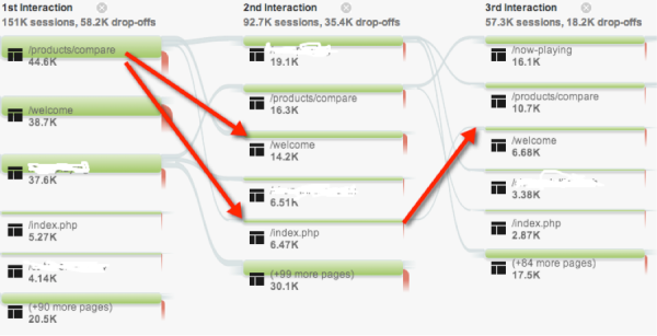
Tools like Google Analytics visitor flows allow slick visualization of user paths and can help to identify common behaviors leading to conversions. Filtering on converting users, it doesn’t require a machine-learning algorithm to see basic patterns in data.

(Click to enlarge.)
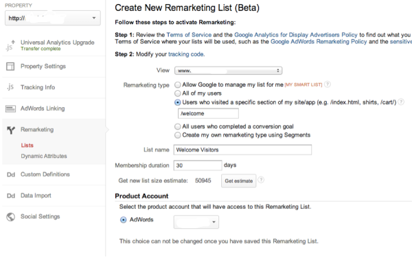
More discrete patterns will require statistical modeling to identify but there is no shame in starting with obvious patterns. If you see a pattern then build a remarketing lists and port is over to AdWords.

(Click to enlarge.)
Leveraging the audience for remarketing, prospecting, and paid search (via Remarketing Lists for Search Ads, aka RLSA, in AdWords) we can isolate users with a known likelihood to convert based on previous actions.
RLSA presents a truly unique opportunity to augment bids and associated ad copy based on a combination of intent (search query) and predicted conversion rate based on user actions (bid). You can quickly imagine a world where we’re segmenting a PPC account into known conversion rate buckets to more intelligently execute bid management.
Conclusion
Hopefully, it’s becoming clear that audiences are not just for remarketing. Just because Google Analytics tells us the audiences we’re building are for remarketing doesn’t mean that’s what we have to use them for. We might find that user that looks at product X and Y are likely to purchase product Z. By all means we should then build a list of users who have looked at X and Y and advertise Z to them.
The creative application of audiences is the future of paid advertising. Fortunately Google provides us with an effective toolset to start building audiences via Google Analytics and an easy solution to port those audiences over to AdWords. I strongly encourage everyone to familiarize themselves with custom audiences.
It all comes together when you merge CLV calculations into audience modeling. It’s as close to direct response panacea that I can imagine. The tools are there, so it’s time to start hacking.


Comments